Learn the most Powerful Formula for Google Spreadsheet.

The Query formula in Google Sheet is quite a powerful and versatile function. So much so that,we can call it a one-stop-shop for all the logical, lookup, summation, counting, averaging, filtering and sorting requirements. It helps us fetch specific information from a data set, through a query statement. Much like fetching result sets from a database using queries. The syntex of the Query language used in this formula is similar to SQL.

SYNTEX

QUERY (data, query, [headers])

data – is the reference to the range of cells on which we want to query upon.

query – is the text using which the QUERY formula churns out the information we are looking for from the data set. Since it is expected to be a string, it has to be enclosed within a set of quotes. Or, it can also be a reference to a cell, where the query text is stored.


headers – is an optional parameter that indicates the number of header rows at the top of the data. If left out, Google Sheets guesses the value based on the content within the data.

Usage: Query Formula

First of all, to understand how the formula is put to use, let us consider the following sample data. It consists of information corresponding to a list of students who have enrolled into various courses at a university. For all the demonstration purposes, we’ll enter the formula in the cell G1. It will be displayed in the formula bar in the snapshots.

Example # 1:

We will start off with a very fundamental demonstration. So, we use the QUERY formula to fetch the names of the students who are residing on campus.

Example # 2:

Having dealt with the basic example, let us now try fetching the names of the students who are NOT residing on campus.

Example # 3:

Now, we will fetch the names, ages, departments of the students whose have taken more than 7 courses.

Example # 4:

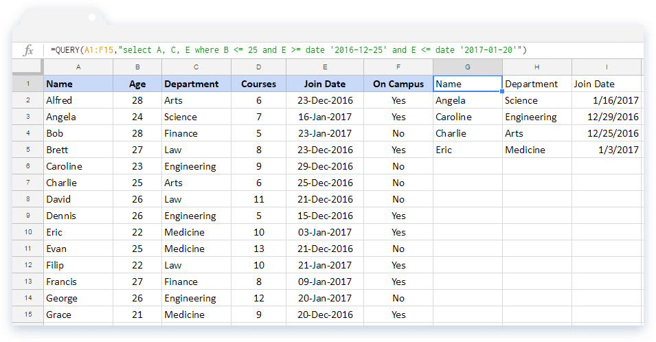
We will now attempt taking this a step further. We bring up the names, departments, join dates of the students aged 25 or below, and have joined the university between 25-Dec-2016 and 20-Jan-2017. Please note, in the query text, the dates always have to go with yyyy-mm-dd format, enclosed within single quotes.

Example # 5:

What if we need to reference the date from a cell? No problem there! We will get around with the help of concatenating operators and a text function. Therefore, in the example below, we will get the names and join dates of the students that joined after 1-Jan-2017.

Example # 6:

Is there a way to list out all of the departments and the display numbers of courses taken from the respective department? Yes, there is! And, we might as well understand the power and versatility that the QUERY formula offers.

You will notice that the QUERY formula returned the second column with the header “sum Courses”. Honestly, it is a bit awkward to have that for a header. But, we can fix that and rename it. Not only that, we will also use the second column (now renamed to ‘Courses Taken’) to sort in ascending order. Here is how we do it.

Example # 7:

Can we display the number of instances of each of the departments? Of course, we can! The QUERY formula got us covered here as well.

Example # 8:

Consequently, we will now experiment with the third parameter. While this is an optional input, it might come in handy when we come across headers that span across multiple rows. In such cases, this parameter helps us combine the headers in one single row, as shown below.

Query function video coming very soon. I explain very easy & simple way to how to use query function to generate amazing report.